Complete AS-AD Model
Unlike the aggregate demand curve, the aggregate supply curve does not usually shift independently. This is because the equation for the aggregate supply curve contains no terms that are indirectly related to either the price level or output. Instead, the equation for aggregate supply contains only terms derived from the AS-AD model. For this reason, to understand how the aggregate supply curve shifts, we must work from the AS-AD model as a whole.

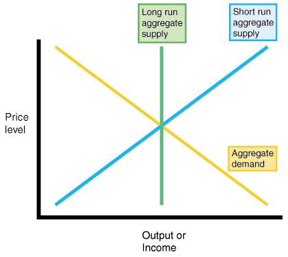
depicts the AS-AD model. The intersection of the short-run aggregate supply curve, the long-run aggregate supply curve, and the aggregate demand curve gives the equilibrium price level and the equilibrium level of output. This is the starting point for all problems dealing with the AS- AD model.
Shifts in Aggregate Demand in the AS-AD Model
The primary cause of shifts in the economy is aggregate demand. Recall that aggregate demand can be affected by consumers both domestic and foreign, the Fed, and the government. For a review of the shifters of aggregate demand, see the SparkNote on aggregate demand. In general, any expansionary policy shifts the aggregate demand curve to the right while any contractionary policy shifts the aggregate demand curve to the left. In the long run, though, since long-term aggregate supply is fixed by the factors of production, short-term aggregate supply shifts to the left so that the only effect of a change in aggregate demand is a change in the price level.

Let's work through an example. For this example, refer to . Notice that we begin at point A where short-run aggregate supply curve 1 meets the long-run aggregate supply curve and aggregate demand curve 1. The point where the short-run aggregate supply curve and the aggregate demand curve meet is always the short-run equilibrium. The point where the long-run aggregate supply curve and the aggregate demand curve meet is always the long-run equilibrium. Thus, we are in long-run equilibrium to begin.
Now say that the Fed pursues expansionary monetary policy. In this case, the aggregate demand curve shifts to the right from aggregate demand curve 1 to aggregate demand curve 2. The intersection of short- run aggregate supply curve 1 and aggregate demand curve 2 has now shifted to the upper right from point A to point B. At point B, both output and the price level have increased. This is the new short-run equilibrium.
But, as we move to the long run, the expected price level comes into line with the actual price level as firms, producers, and workers adjust their expectations. When this occurs, the short-run aggregate supply curve shifts along the aggregate demand curve until the long-run aggregate supply curve, the short-run aggregate supply curve, and the aggregate demand curve all intersect. This is represented by point C and is the new equilibrium where short-run aggregate supply curve 2 equals the long-run aggregate supply curve and aggregate demand curve 2. Thus, expansionary policy causes output and the price level to increase in the short run, but only the price level to increase in the long run.

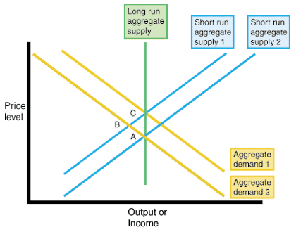
The opposite case exists when the aggregate demand curve shifts left. For example, say the Fed pursues contractionary monetary policy. For this example, refer to . Notice that we begin again at point A where short-run aggregate supply curve 1 meets the long-run aggregate supply curve and aggregate demand curve 1. We are in long-run equilibrium to begin.
If the Fed pursues contractionary monetary policy, the aggregate demand curve shifts to the left from aggregate demand curve 1 to aggregate demand curve 2. The intersection of short-run aggregate supply curve 1 and the aggregate demand curve has now shifted to the lower left from point A to point B. At point B, both output and the price level have decreased. This is the new short-run equilibrium.
But, as we move to the long run, the expected price level comes into line with the actual price level as firms, producers, and workers adjust their expectations. When this occurs, the short-run aggregate supply curve shifts down along the aggregate demand curve until the long-run aggregate supply curve, the short-run aggregate supply curve, and the aggregate demand curve all intersect. This is represented by point C and is the new equilibrium where short-run aggregate supply curve 2 meets the long-run aggregate supply curve and aggregate demand curve 2. Thus, contractionary policy causes output and the price level to decrease in the short run, but only the price level to decrease in the long run.
This is the logic that is applied to all shifts in aggregate demand. The long-run equilibrium is always dictated by the intersection of the vertical long-run aggregate supply curve and the aggregate demand curve. The short-run equilibrium is always dictated by the intersection of the short-run aggregate supply curve and the aggregate demand curve. When the aggregate demand curve shifts, the economy always shifts from the long-run equilibrium to the short-run equilibrium and then back to a new long-run equilibrium. By keeping these rules and the examples above in mind it is possible to interpret the effects of any aggregate demand shift in both the short run and in the long run.
Shifts in Aggregate Supply in the AS-AD Model
Shifts in the short-run aggregate supply curve are much rarer than shifts in the aggregate demand curve. Usually, the short-run aggregate supply curve only shifts in response to the aggregate demand curve. But, when a supply shock occurs, the short-run aggregate supply curve shifts without prompting from the aggregate demand curve. Fortunately, the correction process is exactly the same for a shift in the short-run aggregate supply curve as it is for a shift in the aggregate demand curve. That is, when the short-run aggregate supply curve shifts, a short- run equilibrium exists where the short-run aggregate supply curve intersects the aggregate demand curve. Then the aggregate demand curve shifts along the short-run aggregate supply curve until the aggregate demand curve intersects both the short-run and the long-run aggregate supply curves. Once the economy reaches this new long-run equilibrium, the price level is changed but output is not.
There are two types of supply shocks. Adverse supply shocks include things like increases in oil prices, a drought that destroys crops, and aggressive union actions. In general, adverse supply shocks cause the price level for a given amount of output to increase. This is represented by a shift of the short-run aggregate supply curve to the left. Positive supply shocks include things like decreases in oil prices or an unexpected great crop season. In general, positive supply shocks cause the price level for a given amount of output to decrease. This is represented by a shift of the short-run aggregate supply curve to the right.

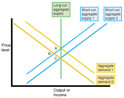
Let's work through an example. For this example, refer to . Notice that we begin at point A where short-run aggregate supply curve 1 meets the long-run aggregate supply curve and aggregate demand curve 1. Thus, we are in long-run equilibrium to begin.
Now say that a positive supply shock occurs: a reduction in the price of oil. In this case, the short-run aggregate supply curve shifts to the right from short-run aggregate supply curve 1 to short-run aggregate supply curve 2. The intersection of short- run aggregate supply curve 2 and aggregate demand curve 1 has now shifted to the lower right from point A to point B. At point B, output has increased and the price level has decreased. This is the new short-run equilibrium.
However, as we move to the long run, aggregate demand adjusts to the new price level and output level. When this occurs, the aggregate demand curve shifts along the short-run aggregate supply curve until the long-run aggregate supply curve, the short-run aggregate supply curve, and the aggregate demand curve all intersect. This is represented by point C and is the new equilibrium where short-run aggregate supply curve 2 equals the long-run aggregate supply curve and aggregate demand curve 2. Thus, a positive supply shock causes output to increase and the price level to decrease in the short run, but only the price level to decrease in the long run.

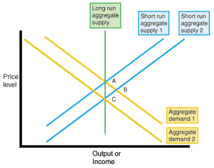
Let's work through another example. For this example, refer to . Notice that we begin at point A where short-run aggregate supply curve 1 meets the long run aggregate supply curve and aggregate demand curve 1. Thus, we are in long-run equilibrium to begin.
Now say that an adverse supply shock occurs: a terrifying increase in the price of oil. In this case, the short-run aggregate supply curve shifts to the left from short-run aggregate supply curve 1 to short-run aggregate supply curve 2. The intersection of short-run aggregate supply curve 2 and aggregate demand curve 1 has now shifted to the upper left from point A to point B. At point B, output has decreased and the price level has increased. This condition is called stagflation. This is also the new short- run equilibrium.
However, as we move to the long run, aggregate demand adjusts to the new price level and output level. When this occurs, the aggregate demand curve shifts along the short-run aggregate supply curve until the long-run aggregate supply curve, the short-run aggregate supply curve, and the aggregate demand curve all intersect. This is represented by point C and is the new equilibrium where short-run aggregate supply curve 2 equals the long-run aggregate supply curve and aggregate demand curve 2. Thus, an adverse supply shock causes output to decrease and the price level to increase in the short run, but only the price level to increase in the long run.
This is the logic that is applied to all shifts in short-run aggregate supply. The long-run equilibrium is always dictated by the intersection of the vertical long run aggregate supply curve and the aggregate demand curve. The short-run equilibrium is always dictated by the intersection of the short-run aggregate supply curve and the aggregate demand curve. When the short-run aggregate supply curve shifts, the economy always shifts from the long-run equilibrium to the short-run equilibrium and then back to a new long-run equilibrium. By keeping these rules and the examples above in mind, it is possible to interpret the effects of any short-run aggregate supply shift, or supply shock, in both the short run and in the long run.
Conclusions from the AS-AD Model
This section has served a number of purposes. First, we covered how and why the short-run aggregate supply curve shifts. Second, we reviewed how and why the aggregate demand curve shifts. Third, we introduced the mechanism that moves the economy from the long run to the short run and back to the long run when there is a change in either aggregate supply or aggregate demand. At this stage, you have the ability to use the highly realistic model of the macroeconomy provided by the AS-AD diagram to analyze the effects of macroeconomic policies. This will prove to be the most powerful tool in your collection for understanding the macroeconomy. Use it wisely!


 payment page


